More plotting with pandas
Things we will cover:
- scatter plots
- histograms
- grouping data
- box-and-whisker plots
- plotting on a map
First, the usual imports…
import matplotlib.pyplot as plt
import pandas as pd
Scatter plots
Let’s use the box office dataset
movie_data = pd.read_csv('all-time-worldwide-box-office.csv')
movie_data.head()
| Rank | Year | Movie | WorldwideBox Office | DomesticBox Office | InternationalBox Office | |
|---|---|---|---|---|---|---|
| 0 | 1 | 2009 | Avatar | 760,507,625 | $2,085,391,916 | |
| 1 | 2 | 2019 | Avengers: Endgame | 858,373,000 | $1,939,427,564 | |
| 2 | 3 | 1997 | Titanic | 659,363,944 | $1,548,622,601 | |
| 3 | 4 | 2015 | Star Wars Ep. VII: The Force Awakens | 936,662,225 | $1,127,953,592 | |
| 4 | 5 | 2018 | Avengers: Infinity War | 678,815,482 | $1,365,725,041 |
Remember, we need to clean those dollar amounts up. This is the same thing we did last time, except we’ll also conver the dollar amounts to billions at the same time.
def clean_money(entry):
    if isinstance(entry, float):
        return 0

return int(entry.strip('$').replace(',', ''))movie_data['Worldwide'] = movie_data['WorldwideBox Office'].apply(clean_money)/1e9
movie_data['Domestic'] = movie_data['DomesticBox Office'].apply(clean_money)/1e9
movie_data['International'] = movie_data['InternationalBox Office'].apply(clean_money)/1e9
movie_data.head()| Rank | Year | Movie | WorldwideBox Office | DomesticBox Office | InternationalBox Office | Worldwide | Domestic | International | |
|---|---|---|---|---|---|---|---|---|---|
| 0 | 1 | 2009 | Avatar | 760,507,625 | $2,085,391,916 | 2.845900 | 0.760508 | 2.085392 | |
| 1 | 2 | 2019 | Avengers: Endgame | 858,373,000 | $1,939,427,564 | 2.797801 | 0.858373 | 1.939428 | |
| 2 | 3 | 1997 | Titanic | 659,363,944 | $1,548,622,601 | 2.207987 | 0.659364 | 1.548623 | |
| 3 | 4 | 2015 | Star Wars Ep. VII: The Force Awakens | 936,662,225 | $1,127,953,592 | 2.064616 | 0.936662 | 1.127954 | |
| 4 | 5 | 2018 | Avengers: Infinity War | 678,815,482 | $1,365,725,041 | 2.044541 | 0.678815 | 1.365725 |
To make a scatter plot, use:
kind='scatter'Scatter plots work well when the values the data can take are granular. For example, no two movies likely have the exact same box office numbers. So let’s scatter year versus worldwide box office. This is a nice way to see what is in the dataset.
movie_data.plot(x='Year', y='Worldwide', kind='scatter',
                ylabel='WorldWide Box Office (billions)', xlabel='Year')
<AxesSubplot:xlabel='Year', ylabel='WorldWide Box Office (billions)'>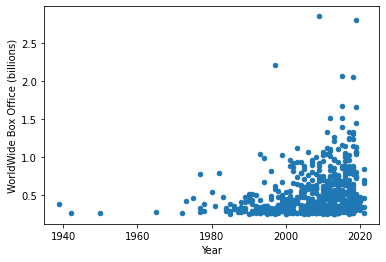
Scatter plots are also useful when you want to see if there is a relationship between two columns in your dataset. For example, if a movie has a high domestic box office, is it likely to also have a high international box office? Let’s do a scatter plot of these two columns.
movie_data.plot(x='Domestic', y='International', kind='scatter',
                xlabel='Domestic Box Office (billions)',
                ylabel='International Box Office (billions)')
<AxesSubplot:xlabel='Domestic Box Office (billions)', ylabel='International Box Office (billions)'>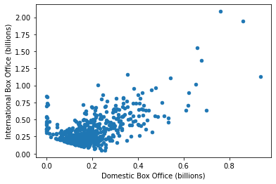
One of the useful things about a scatter plot is we can look for and then examine outliers. What are these movies that have very low International box office numbers?
low_international = movie_data['International'] < 0.1
movie_data[low_international]| Rank | Year | Movie | WorldwideBox Office | DomesticBox Office | InternationalBox Office | Worldwide | Domestic | International | |
|---|---|---|---|---|---|---|---|---|---|
| 407 | 412 | 2000 | How the Grinch Stole Christmas | 260,348,825 | $85,096,578 | 0.345445 | 0.260349 | 0.085097 | |
| 455 | 460 | 1984 | Beverly Hills Cop | 234,760,478 | $81,539,522 | 0.316300 | 0.234760 | 0.081540 | |
| 482 | 487 | 2009 | The Blind Side | 255,959,475 | $49,746,319 | 0.305706 | 0.255959 | 0.049746 | |
| 505 | 511 | 2002 | Austin Powers in Goldmember | 213,117,789 | $83,220,874 | 0.296339 | 0.213118 | 0.083221 | |
| 508 | 514 | 1984 | Ghostbusters | 242,212,467 | $52,999,344 | 0.295212 | 0.242212 | 0.052999 | |
| 530 | 536 | 2005 | Wedding Crashers | 209,218,368 | $74,000,000 | 0.283218 | 0.209218 | 0.074000 | |
| 552 | 558 | 2012 | Lincoln | 182,207,973 | $91,138,308 | 0.273346 | 0.182208 | 0.091138 |
What about those movies that have very high Domestic box office numbers (all of them also doing quite well internationally)?
outliers = movie_data['Domestic'] > 0.6
movie_data[outliers]| Rank | Year | Movie | WorldwideBox Office | DomesticBox Office | InternationalBox Office | Worldwide | Domestic | International | |
|---|---|---|---|---|---|---|---|---|---|
| 0 | 1 | 2009 | Avatar | 760,507,625 | $2,085,391,916 | 2.845900 | 0.760508 | 2.085392 | |
| 1 | 2 | 2019 | Avengers: Endgame | 858,373,000 | $1,939,427,564 | 2.797801 | 0.858373 | 1.939428 | |
| 2 | 3 | 1997 | Titanic | 659,363,944 | $1,548,622,601 | 2.207987 | 0.659364 | 1.548623 | |
| 3 | 4 | 2015 | Star Wars Ep. VII: The Force Awakens | 936,662,225 | $1,127,953,592 | 2.064616 | 0.936662 | 1.127954 | |
| 4 | 5 | 2018 | Avengers: Infinity War | 678,815,482 | $1,365,725,041 | 2.044541 | 0.678815 | 1.365725 | |
| 5 | 6 | 2015 | Jurassic World | 652,306,625 | $1,017,673,342 | 1.669980 | 0.652307 | 1.017673 | |
| 8 | 9 | 2012 | The Avengers | 623,357,910 | $891,742,301 | 1.515100 | 0.623358 | 0.891742 | |
| 11 | 12 | 2018 | Black Panther | 700,059,566 | $636,434,755 | 1.336494 | 0.700060 | 0.636435 | |
| 13 | 14 | 2017 | Star Wars Ep. VIII: The Last Jedi | 620,181,382 | $711,453,759 | 1.331635 | 0.620181 | 0.711454 | |
| 17 | 18 | 2018 | Incredibles 2 | 608,581,744 | $634,223,615 | 1.242805 | 0.608582 | 0.634224 |
Histograms
A histogram let’s us visualize how many things meet certain criteria. For
examle, how many movies manage to make a billion at the box office? We can do a
histogram on the worldwide box office to see this. To create a histogram, you
can use hist() on a single column or an entire data frame:
movie_data.hist(figsize=(10,10)) array([[<AxesSubplot:title={'center':'Rank'}>,
<AxesSubplot:title={'center':'Year'}>],
[<AxesSubplot:title={'center':'Worldwide'}>,
<AxesSubplot:title={'center':'Domestic'}>],
[<AxesSubplot:title={'center':'International'}>, <AxesSubplot:>]],
dtype=object)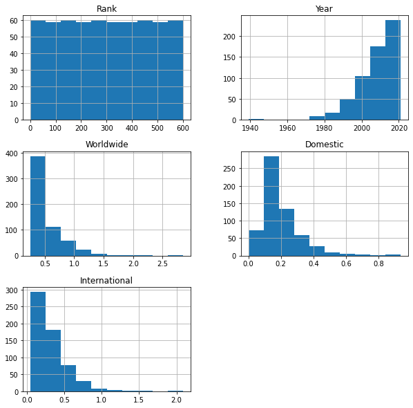
movie_data.hist(column='Worldwide') array([[<AxesSubplot:title={'center':'Worldwide'}>]], dtype=object)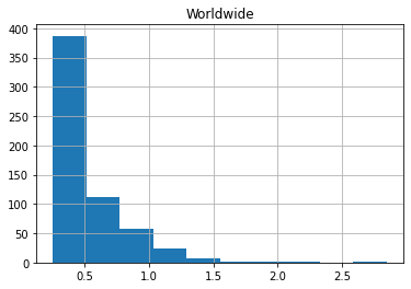
To put labels on the axes of this plot, we need to use matplotlib because they
don’t work inside of hist():
movie_data.hist(column='Worldwide')
plt.xlabel('Worldwide Box Office (billions)')
plt.ylabel('Number of Movies')
plt.title('Histogram of Worldwide Box Office')
Text(0.5, 1.0, 'Histogram of Worldwide Box Office')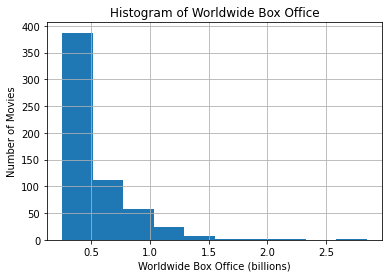
We can specify the number of bins to use in the histogram
movie_data.hist(column='Worldwide',bins=20)
plt.xlabel('Worldwide Box Office (billions)')
plt.ylabel('Number of Movies')
plt.title('Histogram of Worldwide Box Office')
Text(0.5, 1.0, 'Histogram of Worldwide Box Office')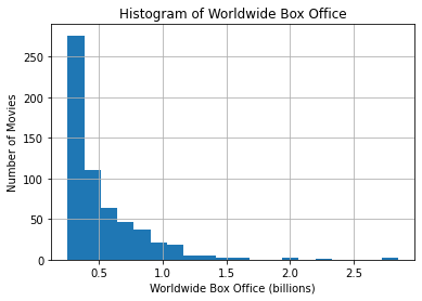
We can specify the exact bins to use:
movie_data.hist(column='Worldwide', bins=[0,0.5,1,1.5,2,2.5,3])
plt.xlabel('Worldwide Box Office (billions)')
plt.ylabel('Number of Movies')
plt.title('Histogram of Worldwide Box Office')
Text(0.5, 1.0, 'Histogram of Worldwide Box Office')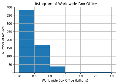
Grouping Data
When you have data that is categorical — it takes a discrete set of values — you may want to group the data according to these values.
What are you going to do with the data once it is grouped? Maybe you want to look at the mean or max or min money earned by all the movies released each year.
Let’s group all of our movies by the year they were released and look at their mean box office:
means_per_year = movie_data.groupby('Year').mean().reset_index()
means_per_year.head()
| Year | Rank | Worldwide | Domestic | International | |
|---|---|---|---|---|---|
| 0 | 1939 | 319.0 | 0.390525 | 0.198680 | 0.191845 |
| 1 | 1942 | 571.0 | 0.268000 | 0.102797 | 0.165203 |
| 2 | 1950 | 585.0 | 0.263591 | 0.085000 | 0.178591 |
| 3 | 1965 | 533.0 | 0.286214 | 0.163214 | 0.123000 |
| 4 | 1972 | 568.0 | 0.268500 | 0.134966 | 0.133534 |
Notice that we used reset_index() to get Year added as a column.
Now we can plot this:
recent = means_per_year['Year'] > 2000
means_per_year[recent].plot(x='Year', y='Worldwide', ylabel='Mean Worldwide Box Office (billions)', )
<AxesSubplot:xlabel='Year', ylabel='Mean Worldwide Box Office (billions)'>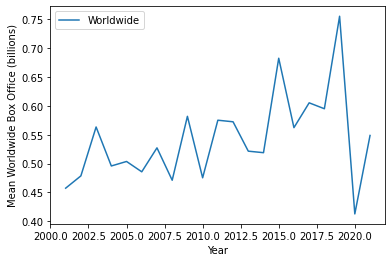
We can also look at the total box office of all movies released each year, using
sum():
total_per_year = movie_data.groupby('Year').sum().reset_index()
total_per_year.head()
| Year | Rank | Worldwide | Domestic | International | |
|---|---|---|---|---|---|
| 0 | 1939 | 319 | 0.390525 | 0.198680 | 0.191845 |
| 1 | 1942 | 571 | 0.268000 | 0.102797 | 0.165203 |
| 2 | 1950 | 585 | 0.263591 | 0.085000 | 0.178591 |
| 3 | 1965 | 533 | 0.286214 | 0.163214 | 0.123000 |
| 4 | 1972 | 568 | 0.268500 | 0.134966 | 0.133534 |
Now we can plot this:
total_per_year.plot(x='Year', y='Worldwide', ylabel='Total Box Office') <AxesSubplot:xlabel='Year', ylabel='Total Box Office'>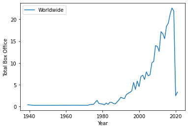
Box-and-whisker plots
A box-and-whisker plot is useful for exploring multiple statistics that characterize a distribution of values.
We can divide all the data into quartiles — four segments that each contain 25% of the data:
- Q1 is the 25th-percentile. 25% of the data is below that point.
- Q2 is the 50th-percentile — the median. Half of the data is at or below that point, and half above it.
- Q3 is the 75th percentile. 75% of the data is below that point.
A box plot shows all three of these.
Let’s create a box-and-whisker plot that shows statistics about the worldwide box office for movies since the year 2000.
recent = movie_data['Year'] > 2000
means = movie_data[recent].groupby('Year').mean()
means.boxplot(column=['Worldwide','International','Domestic'])
<AxesSubplot:>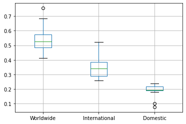
-
The bottom of the box is Q1, the top of the box is Q3.
-
The middle line is the Q2, the median.
-
The distance between Q3 and Q1 is the interquartile range (IQR).
-
Each whisker extends to the furthest data point that is within 1.5 times the IQR.
-
Dots are outliers
Use box plots carefully. These two histograms have the same box-and-whiskers plot.

You really should use a violin plot instead of a box-and-whiskers plot. But for that you should use seaborn.
import seaborn as sns

recent_movies = movie_data[recent]
sns.violinplot(data=recent_movies, y="Worldwide")
<AxesSubplot:ylabel='Worldwide'>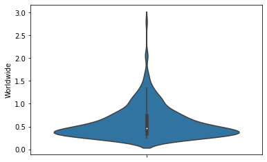
In the world of Python plotting:
- matplotlib — does everything, low level
- pandas — uses dataframes, built on matplotlib, can always use matplotlib to tweak
- seaborn — tries to do a small number of things well, and make them look pretty
We won’t spend time on violin plots here. Go here if you want to learn more about violin plots.
You can plot lots of box plots at once using by inside of boxplot():
recent = movie_data['Year'] > 2010
movie_data[recent].boxplot(by="Year", column='Worldwide', figsize=(8,5))
# Because we are plotting a bunch of things, we have  both 'suptitle' and 'title' available
plt.suptitle('Worldwide Box Office')
plt.title('')
plt.ylabel('Worldwide Box Office (billions)')
Text(0, 0.5, 'Worldwide Box Office (billions)')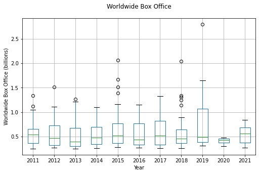
import seaborn as sns

recent_movies = movie_data[recent]
fig, ax = plt.subplots(figsize=(12, 5))
sns.violinplot(data=recent_movies, x="Year", y="Worldwide", ax=ax)
<AxesSubplot:xlabel='Year', ylabel='Worldwide'>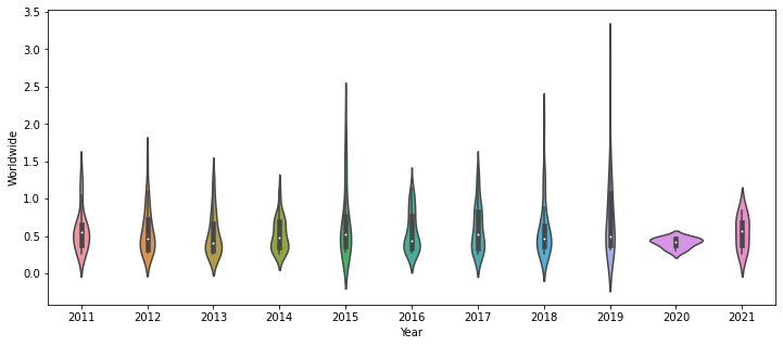
Plotting on a map of the world
Let’s use a new data set — one that includes oil spills and their locations.
Let’s take a look at the dataset:
! head incidents.csvIt has lots of empty data points!
oil_spills = pd.read_csv('incidents.csv')
oil_spills.head()| id | open_date | name | location | lat | lon | threat | tags | commodity | measure_skim | measure_shore | measure_bio | measure_disperse | measure_burn | max_ptl_release_gallons | posts | description | |
|---|---|---|---|---|---|---|---|---|---|---|---|---|---|---|---|---|---|
| 0 | 10431 | 2022-03-21 | Tug Vessel Loses Power, Grounds, and Leaks Die… | Neva Strait, Sitka, AK | 57.270000 | -135.593330 | Oil | NaN | NaN | NaN | NaN | NaN | NaN | NaN | NaN | 0 | At approximately 0400 on 21-Mar02922, the tug … |
| 1 | 10430 | 2022-03-17 | Compromised Fuel Transfer Pipe Spills Oil into… | Oswego, NY | 43.459410 | -76.531650 | Oil | NaN | NaN | NaN | NaN | NaN | NaN | NaN | NaN | 0 | On March 17, 2022, NOAA ERD was notified by Mi… |
| 2 | 10429 | 2022-03-16 | Floating Humpback Whale Carcass off of Carolin… | Carolina Beach, NC, USA | 34.031323 | -77.830343 | Other | NaN | NaN | NaN | NaN | NaN | NaN | NaN | NaN | 0 | On March 16, 2022, the Gulf of Mexico Marine M… |
| 3 | 10428 | 2022-03-15 | Containership Grounded off Gibson Island in Ch… | Gibson Island, MD, USA | 39.070000 | -76.410000 | Oil | NaN | NaN | NaN | NaN | NaN | NaN | NaN | NaN | 2 | On 15 March 2022, USCG Sector Maryland NCR not… |
| 4 | 10426 | 2022-03-14 | Oil Pipeline Discharge into Cahokia Canal, Edw… | Cahokia Canal, Edwardsville, IL | 38.824034 | -89.974600 | Oil | NaN | NaN | NaN | NaN | NaN | NaN | NaN | NaN | 0 | On March 14, 2022, USEPA Region 5 contacted th… |
Let’s create a simple scatter plot using latitude and longitude.
oil_spills.plot(x="lon", y="lat", kind="scatter", xlabel='Longitude', ylabel='Latitude', title='Oil Spills')
<AxesSubplot:title={'center':'Oil Spills'}, xlabel='Longitude', ylabel='Latitude'>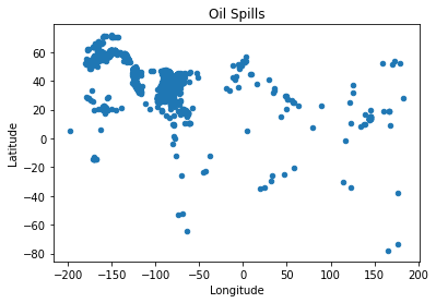
This looks a little bit like the United States. What if we put a real map behind it?
🌎🐼
pip install geopandasimport geopandas as gpd
countries = gpd.read_file(gpd.datasets.get_path("naturalearth_lowres"))
# plot the countries first
countries.plot(color="lightgrey")
# now plot the oil spills
# use ax=plt.gca() to get it on the same plot
# use figsize to get a good shape
oil_spills.plot(x="lon", y="lat", kind="scatter", ax=plt.gca(),figsize=(100,70))
<AxesSubplot:xlabel='lon', ylabel='lat'>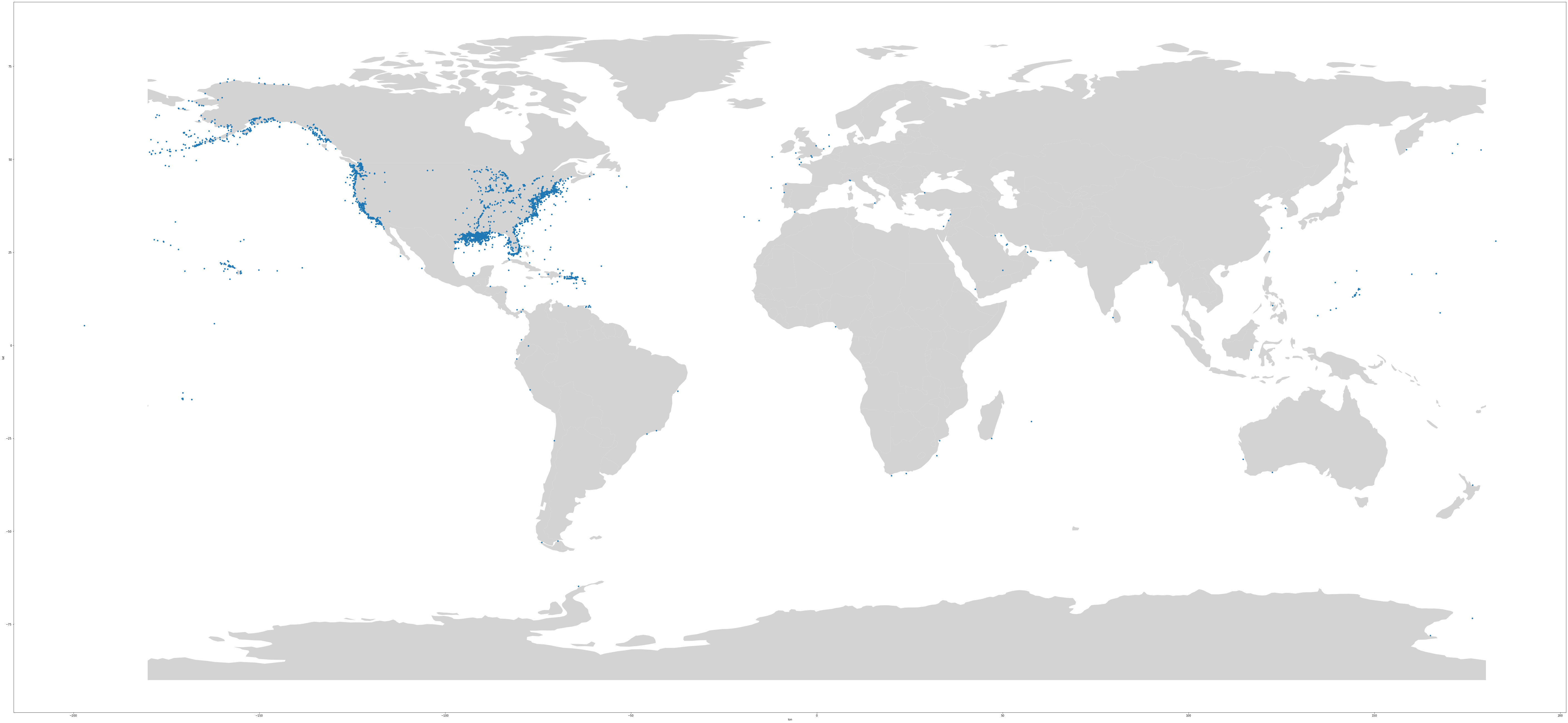
That’s pretty good, but what if we want to only plot North and South America?
subset = countries.continent.isin(['North America','South America'])countries = gpd.read_file(
gpd.datasets.get_path("naturalearth_lowres"))
# get just the countries we want to plot
subset = countries.continent.isin(['North America','South America'])
countries[subset].plot(color="lightgrey")
oil_spills.plot(x="lon", y="lat", kind="scatter", ax=plt.gca(),figsize=(20,15), s=1, color='firebrick')
<AxesSubplot:xlabel='lon', ylabel='lat'>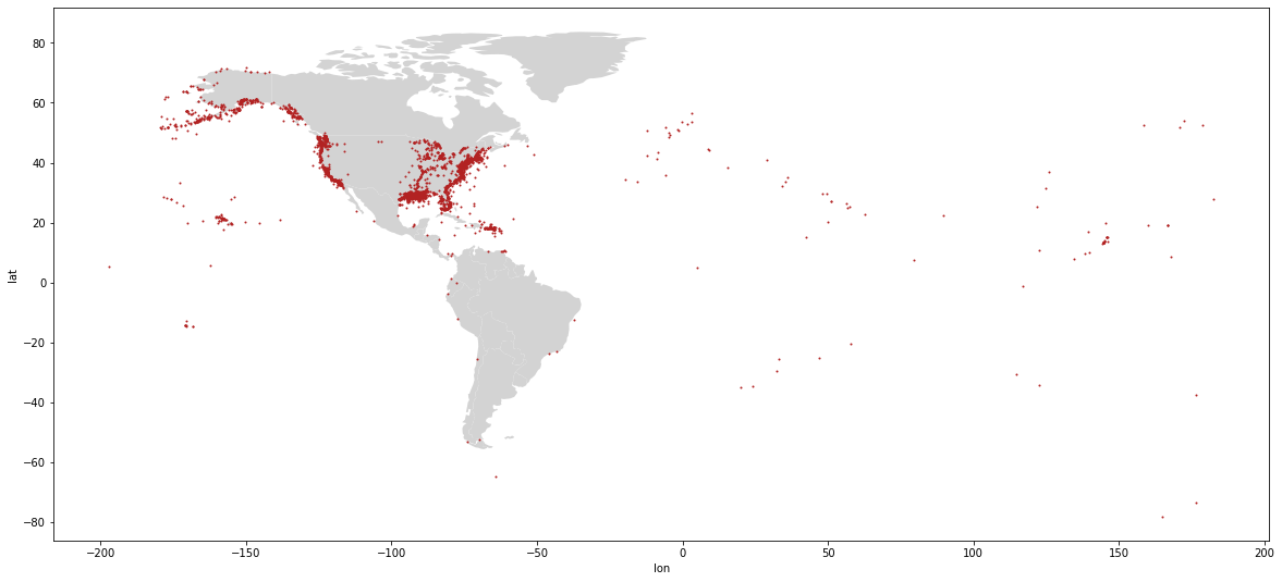
What if we want to zoom in on just the continental United States? Use these
parameters in plot()
ylim=(start,end)
xlim=(start,end)
countries = gpd.read_file(gpd.datasets.get_path("naturalearth_lowres"))
subset = countries.continent.isin(['North America'])
countries[subset].plot(color="lightgrey")
oil_spills.plot(x="lon", y="lat", kind="scatter", ax=plt.gca(),figsize=(20,15),
s=1, color='firebrick', ylim=(10,55), xlim=(-150,-50))
<AxesSubplot:xlabel='lon', ylabel='lat'>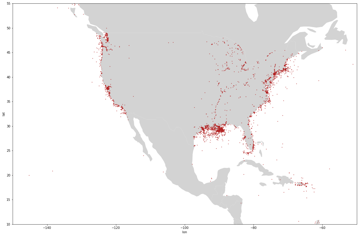
Let’s do it all over again
We’ll read in the Chicago beach water monitoring data
chicago = pd.read_csv("bwq.csv", parse_dates=['Measurement Timestamp'])
chicago.head()
| Beach Name | Measurement Timestamp | Water Temperature | Turbidity | Transducer Depth | Wave Height | Wave Period | Battery Life | Measurement Timestamp Label | Measurement ID | |
|---|---|---|---|---|---|---|---|---|---|---|
| 0 | Montrose Beach | 2013-08-30 08:00:00 | 20.3 | 1.18 | 0.891 | 0.080 | 3.0 | 9.4 | 8/30/2013 8:00 AM | MontroseBeach201308300800 |
| 1 | Ohio Street Beach | 2016-05-26 13:00:00 | 14.4 | 1.23 | NaN | 0.111 | 4.0 | 12.4 | 05/26/2016 1:00 PM | OhioStreetBeach201605261300 |
| 2 | Calumet Beach | 2013-09-03 16:00:00 | 23.2 | 3.63 | 1.201 | 0.174 | 6.0 | 9.4 | 9/3/2013 4:00 PM | CalumetBeach201309031600 |
| 3 | Calumet Beach | 2014-05-28 12:00:00 | 16.2 | 1.26 | 1.514 | 0.147 | 4.0 | 11.7 | 5/28/2014 12:00 PM | CalumetBeach201405281200 |
| 4 | Montrose Beach | 2014-05-28 12:00:00 | 14.4 | 3.36 | 1.388 | 0.298 | 4.0 | 11.9 | 5/28/2014 12:00 PM | MontroseBeach201405281200 |
Then we need to drop any invalid measurements:
chicago = chicago.dropna(subset=['Measurement Timestamp'])and add a column for the year:
chicago = chicago.dropna(subset=['Measurement Timestamp'])

def get_year(date):
    return int(date.year)

chicago['Year'] = chicago['Measurement Timestamp'].apply(get_year)
chicago.head()| Beach Name | Measurement Timestamp | Water Temperature | Turbidity | Transducer Depth | Wave Height | Wave Period | Battery Life | Measurement Timestamp Label | Measurement ID | Year | |
|---|---|---|---|---|---|---|---|---|---|---|---|
| 0 | Montrose Beach | 2013-08-30 08:00:00 | 20.3 | 1.18 | 0.891 | 0.080 | 3.0 | 9.4 | 8/30/2013 8:00 AM | MontroseBeach201308300800 | 2013 |
| 1 | Ohio Street Beach | 2016-05-26 13:00:00 | 14.4 | 1.23 | NaN | 0.111 | 4.0 | 12.4 | 05/26/2016 1:00 PM | OhioStreetBeach201605261300 | 2016 |
| 2 | Calumet Beach | 2013-09-03 16:00:00 | 23.2 | 3.63 | 1.201 | 0.174 | 6.0 | 9.4 | 9/3/2013 4:00 PM | CalumetBeach201309031600 | 2013 |
| 3 | Calumet Beach | 2014-05-28 12:00:00 | 16.2 | 1.26 | 1.514 | 0.147 | 4.0 | 11.7 | 5/28/2014 12:00 PM | CalumetBeach201405281200 | 2014 |
| 4 | Montrose Beach | 2014-05-28 12:00:00 | 14.4 | 3.36 | 1.388 | 0.298 | 4.0 | 11.9 | 5/28/2014 12:00 PM | MontroseBeach201405281200 | 2014 |
Let’s try doing a scatter plot of wave height and wave period to see if they are related:
chicago.plot(x='Wave Period', y='Wave Height', kind='scatter') <AxesSubplot:xlabel='Wave Period', ylabel='Wave Height'>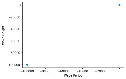
Oops! Looks like we have some negative wave heights and periods! Let’s clean our data:
clean_chicago = chicago[(chicago['Wave Height'] > 0) & (chicago['Wave Period'] > 0)]
clean_chicago.plot(x='Wave Period', y='Wave Height', kind='scatter')
<AxesSubplot:xlabel='Wave Period', ylabel='Wave Height'>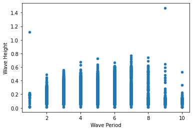
We can do the same thing with wave period and Turbidity.
clean_chicago.plot(x='Wave Period', y='Turbidity', kind='scatter') <AxesSubplot:xlabel='Wave Period', ylabel='Turbidity'>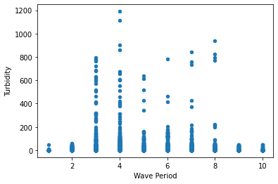
This is a line plot, but for fun, let’s look at wave height over time at a certain beach:
recent = clean_chicago['Year'] == 2016
montrose = clean_chicago['Beach Name'] == 'Montrose Beach'
clean_chicago[recent & montrose].plot(x='Measurement Timestamp', y='Wave Height')
<AxesSubplot:xlabel='Measurement Timestamp'>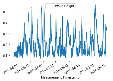
How about a histogram so we can see how common various wave heights are?
clean_chicago[recent & montrose].hist(column='Wave Height') array([[<AxesSubplot:title={'center':'Wave Height'}>]], dtype=object)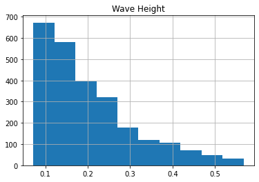
A box plot would give us some statistical data about wave heights:
earlier = clean_chicago['Year'] == 2014
clean_chicago[earlier].groupby('Beach Name').boxplot(column='Wave Height', figsize=(6,18))
63rd Street Beach AxesSubplot(0.1,0.679412;0.363636x0.220588)
Calumet Beach AxesSubplot(0.536364,0.679412;0.363636x0.220588)
Montrose Beach AxesSubplot(0.1,0.414706;0.363636x0.220588)
Ohio Street Beach AxesSubplot(0.536364,0.414706;0.363636x0.220588)
Osterman Beach AxesSubplot(0.1,0.15;0.363636x0.220588)
Rainbow Beach AxesSubplot(0.536364,0.15;0.363636x0.220588)
dtype: object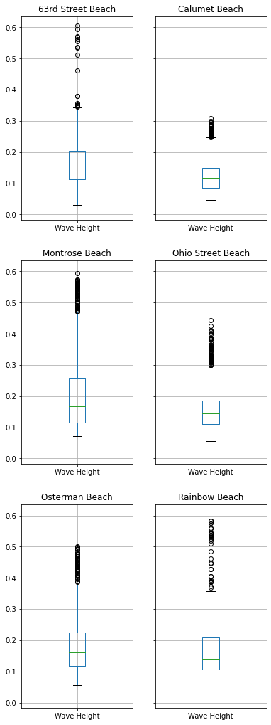
Or we could put those all on one graph:
clean_chicago[earlier].boxplot(by='Beach Name',column='Wave Height', figsize=(10,5)) <AxesSubplot:title={'center':'Wave Height'}, xlabel='Beach Name'>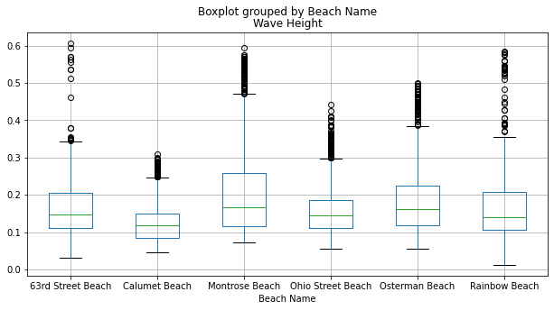
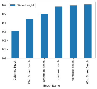
Finally, we can use groupby to compute max wave heights and see which beach
has the highest wave:
grouped = clean_chicago[earlier].groupby('Beach Name').max().sort_values('Wave Height').reset_index()
grouped.plot(x = 'Beach Name', y='Wave Height', kind='bar')
<AxesSubplot:xlabel='Beach Name'>